See also: Analysis View, Expressions, Examples of Expressions
The Time-Series Wizard is a tool that helps you construct the various
time-series expressions supported by LEAP's Analysis
View. These expressions include functions for interpolation, step
functions, smooth curves and linear, exponential and logistic projections.
The wizard is divided into three pages, which you step through using the
Next ( ) and
Previous (
) and
Previous ( )
buttons.
)
buttons.
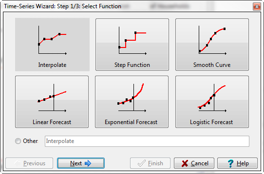
Use this page to select the type of function you want to create. The functions are summarized in graph form on screen as shown below, and are grouped into two main types. The functions on the top row allow you to specify data points for various future years, and the function then calculates the values for intervening years:
The interpolation function calculates values based on a linear (straight line) interpolation between the values you specify.
The step function assumes that values change discretely at the specified data years. In other words, values stay constant after a specified data year, until the next specified data year.
The smooth curve function calculates a best-fit smooth curve based on a polynomial least-squares fit of the specified data points. To achieve a good fit, the smooth curve function requires at least 3 data points.
The interpolation and smooth curve functions are most useful when you expect data to change gradually (for example when modeling the gradual penetration of some common device such as refrigerators or vehicles). The step function is most useful for specifying "lumpy" changes to the energy system, such as the addition of specific power plants to an electric generation system.
The functions on the bottom row, allow you to specify historic data values (i.e. values before the base year). The different functions are then used to extrapolate data forward to calculate future values. Extrapolations are based on linear, exponential or logistic least-squares curve fits. Use these functions with care. The onus is on you to ensure that the projections are reasonable, both in terms of how a) well the estimated curve fits the historical data, and b) how policies and other structural factors may change in the future. In other words, be sure to consider how well you can identify past trends, but also if it is reasonable to expect these past trends to continue into the future. LEAP helps you with task a) by providing various statistics describing the curve-fit: the R2 value, the standard error, and the number of observations. If you need to do a more detailed analysis, we suggest you use the data analysis features built-in to Microsoft Excel, and then link your results to your LEAP analysis (see below).
On page 2 shown below, you select the source of the data for the expression . Select whether you want to enter the data directly (i.e. type it in) or whether you want to link to the values in an external Excel spreadsheet.
Depending on you choice on page 2, in page 3 you either enter the data used by the function using the data table on the left-hand side of the wizard, or you select an Excel spreadsheet and range(s) from which to extract the data for the selected time-series function. The data you is previewed on the right-hand side of the wizard both as a chart and also as the expression that will be used in LEAP.
When entering data
directly, use the Add ( )
and Delete (
)
and Delete ( ) buttons
to add or delete new year/value pairs, or click and drag data points
on the adjoining graph to edit values graphically. For the Interpolation
function, an additional data field is shown allowing you to specify
a percentage growth rate, which is applied after the last specified
data year. By default this value is zero. In other words, by default
values are not extrapolated past the last interpolation data year.
The data you enter will be shown as the points on the preview chart,
while the line drawn on the chart will reflect the projection method
you are using.
) buttons
to add or delete new year/value pairs, or click and drag data points
on the adjoining graph to edit values graphically. For the Interpolation
function, an additional data field is shown allowing you to specify
a percentage growth rate, which is applied after the last specified
data year. By default this value is zero. In other words, by default
values are not extrapolated past the last interpolation data year.
The data you enter will be shown as the points on the preview chart,
while the line drawn on the chart will reflect the projection method
you are using.
In Current Accounts, when creating a linear or exponential regression, an additional check box will be displayed giving you the option of forcing the regression curve through the base year value.
When linking to a Microsoft Excel sheet, a slightly different screen will be displayed. On this screen, first enter the name of the worksheet file (.xls or .xlsx) or use "..." button to browse for the file. Next enter the range or ranges from which the data will be extracted, or click the button attached to the field to select from any named ranges in the worksheet. Ranges can be specified either as names, or as Excel range formulae (e.g. Sheet1!A1:B16).
When taking data from Excel, you can specify either a single range structured as 2 columns or 2 rows of data, in which the first column or row is years and the second column or row is values. Alternatively you can specify two ranges each of which contains a single row or a single column of data. In this case, the first range should contain years and the second range should contain values. Some of the values may be blank reflecting missing data. In all cases, the data must be organized in chronological order (from left to right or from top to bottom. When specifying two ranges, both ranges must be of equal size (ie. have the same number of rows or columns).
Click on the Get Excel Data button to extract the data from Excel and preview the values in the adjoining graph. The points on the chart will be the values in the Excel spreadsheet, while the line drawn on the chart will reflect the projection method you chose on page one. We suggest that you store any subsidiary Excel worksheets in the same folder as your LEAP area data (ie under the My Documents\LEAP2011 Areas\Area Name folder). By using this approach, your Excel worksheets will be copied, backed-up and restored along with all the other area data.
Use the Create Expression As radio buttons to choose how the data should be inserted into the expression you are editing: either as a live Excel link, which will be updated whenever the spreadsheet is edited and saved, or as data, which is initially copied from Excel, but will not subsequently be updated if the Excel spreadsheet is changed. Creating links to Excel spreadsheets is a good approach if you wish to do most of your editing work in Excel, or if you wish to conduct additional modeling outside of LEAP. However, it will also slow down LEAP calculations.
Once you have selected an Excel worksheet
and range, you can click on the large Excel button ( )
to open a copy of Excel and preview the worksheet and range.
)
to open a copy of Excel and preview the worksheet and range.